Streaming platforms are optimised to help you discover new content however there aren't many features to help you manage your existing library. Hitting shuffle on your entire library often results in disjointed listening experience and maintaining playlists can be a pain.
Let's see if we can leverage some machine learning to automate playlist creation.
import pandas as pd
import matplotlib.pyplot as plt
from sklearn.decomposition import PCA
from sklearn.preprocessing import MinMaxScaler
from sklearn.cluster import KMeans
Data
For our dataset we'll use the Spotify top 100 from 2017 available here. Let's take a look at the data
data = pd.read_csv("featuresdf.csv")
data.head(2)
| id | name | artists | danceability | energy | key | loudness | mode | speechiness | acousticness | instrumentalness | liveness | valence | tempo | duration_ms | time_signature |
|---|---|---|---|---|---|---|---|---|---|---|---|---|---|---|---|
| 7qiZfU4dY1lWllzX7mPBI | Shape of You | Ed Sheeran | 0.825 | 0.652 | 1.0 | -3.183 | 0.0 | 0.0802 | 0.5810 | 0.000000 | 0.0931 | 0.931 | 95.977 | 233713.0 | 4.0 |
| 5CtI0qwDJkDQGwXD1H1cL | Despacito - Remix | Luis Fonsi | 0.694 | 0.815 | 2.0 | -4.328 | 1.0 | 0.1200 | 0.2290 | 0.000000 | 0.0924 | 0.813 | 88.931 | 228827.0 | 4.0 |
We can see that the Spotify API exposes a number of audio features for a track, some are obvious like loudness and other's more ambiguous like energy, an explanation of the features can be found here.
we'll use a subset of the features available in the data-set
# Create feature matrix
song_features = ["energy", "liveness","key","tempo",
                "valence", "loudness", "speechiness",
                "acousticness", "danceability",
                "instrumentalness"]
X = data[song_features].values

# Normalise features
scaler = MinMaxScaler()
X = scaler.fit_transform(X)
Dimensionality Reduction
In order to get a visual representation we need to reduce the high dimensional data to a lower dimensional representation using a manifold learning algorithm, the most popular and the one we'll be using is Principal Component Analysis or PCA, which is effectively computing the eigenvectors of our dataset and selecting the most prominent ones (highest eigenvalue) — A more in depth explanation can be found in this article.
pca = PCA(n_components=10)
X_pca = pca.fit_transform(X)
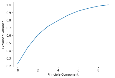
We can look into how the variance of the dataset is represented by the principle components.
explainedVariance = pca.explained_variance_ratio_.cumsum()
plt.plot(range(len(explainedVariance)),explainedVariance)

We see that the first 2 components only represent 44% of the total variance of the data and the way in which the graph increases suggests that the features aren't highly correlated with each other.
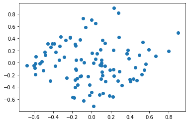
Let's take a look at the scatter plot for the first 2 principal components where each data point represents a song.
plt.scatter(X_pca[:,0],X_pca[:,1])

There aren't a lot of clear clusters that are apparent from this scatter plot, it doesn't give a clear indication as to how we might split the data into different playlists
Clustering
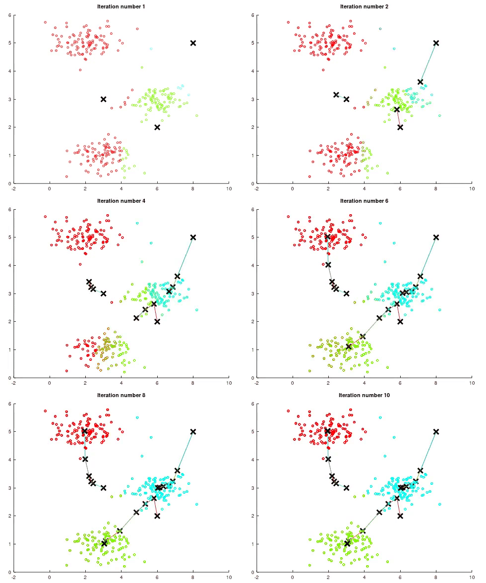
To partition the data into separate playlists we'll use k-means clustering which is the simplest clustering algorithm. It works by randomly initialising cluster centroids and classifying a data point according whichever centroid it's closest to, recomputing cluster centroids and then repeating the process again.

While K-Means is an unsupervised learning algorithm we need to provide the number of desired cluster, there's as an art to picking the number of clusters, you can use the elbow method, 5 playlists from a 100 songs seemed reasonable to me.
kmeans = KMeans(n_clusters=5).fit(X_pca)
centroids = kmeans.cluster_centers_
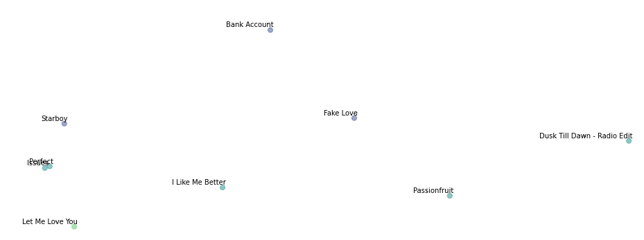
After computing k-means on the high dimensional dataset we can see how some of the songs have been clustered together by colour.

Here is an example of one of the playlists generated.
| name | artists |
|---|---|
| Mask Off | Future |
| Starboy | The Weeknd |
| Location | Khalid |
| Fake Love | Drake |
| DNA. | Kendrick Lamar |
| How Far I'll Go - From "Moana" | Alessia Cara |
| Bank Account | 21 Savage |
Conclusion
The results are meh, you get some fairly anomalous tracks - How Far I'll Go - From "Moana" ? K-means is very sensitive to outliers which can distort the consistency of your clusters. Improvement could be made on the clustering by using an algorithm like HDBSCAN or by using a supervised learning method. Ultimately I don't think spotify relies too heavily on just audio features for it's recommendation system but rather opts for a collaborative filtering approach.